No, the derivative isn’t really an afterthought. Along with the integral it is, in fact, one of the most powerful and useful mathematical objects ever devised and we’ve been working very hard to provide a solid, rigorous foundation for it. In that sense it is a primary focus of our investigations.
On the other hand, now that we have built up all of the machinery we need to define and explore the concept of the derivative it will appear rather pedestrian alongside ideas like the convergence of power series, Fourier series, and the bizarre properties of \(\QQ\) and \(\RR\text{.}\)
You spent an entire semester learning about the properties of the derivative and how to use them to explore the properties of functions so we will not repeat that effort here. Instead we will define it formally in terms of the ideas and techniques we’ve developed thus far.
The derivative is defined at a point. If it is defined at every point in an interval \((a,b)\) then we say that the derivative exists at every point on the interval.
Since it is defined as a limit, Corollary 8.3.5 applies. That is, \(f^\prime(x)\) exists if and only if \(\forall \text{ sequences } (h_n),\, h_n\ne
0\text{,}\) if \(\limit{n}{\infty}{h_n}=0\) then
As we mentioned, the derivative is an extraordinarily useful mathematical tool but it is not our intention to learn to use it here. Our purpose here is to define it rigorously (done) and to show that our formal definition does in fact recover the useful properties you came to know and love in your calculus course.
Suppose \(f\) is differentiable in some interval \((a,b)\) containing \(c\text{.}\) If \(f(c)\ge f(x)\) for every \(x\) in \((a,b)\text{,}\) then \(f^\prime(c)=0\text{.}\)
Since \(f^\prime(c)\) exists we know that if \(\left(h_n\right)_{n=1}^\infty\) converges to zero then the sequence \(a_n =
\frac{f\left(c+h_n\right)-f(c)}{h_n}\) converges to \(f^\prime(c)\text{.}\) The proof consists of showing that \(f^\prime(c)\leq 0\)and that \(f^\prime(c)\geq 0\) from which we conclude that \(f^\prime(c)= 0\text{.}\) We will only show the first part. The second is left as an exercise.
Let \(n_0\) be sufficiently large that \(\frac{1}{n_0}\lt
b-c\) and take \(\left(h_n\right)=\left(\frac{1}{n}\right)_{n=n_0}^\infty\text{.}\) Then \(f\left(c+\frac1n\right)-f(c) \leq 0\) and \(\frac1n>0\text{,}\) so that
However, it would be difficult to prove the MVT right now. So we will first state and prove Rolle’s Theorem, which can be seen as a special case of the MVT. The proof of the MVT will then follow easily.
Michel Rolle first stated the following theorem in 1691. Given this date and the nature of the theorem it would be reasonable to suppose that Rolle was one of the early developers of calculus but this is not so. In fact, Rolle was disdainful of both Newton and Leibniz’s versions of calculus, once deriding them as a collection of “ingenious fallacies.” It is a bit ironic that his theorem is so fundamental to the modern development of the calculus he ridiculed.
Since \(f\) is continuous on \([a,b]\) we see, by the Extreme Value Theorem, that \(f\) has both a maximum and a minimum on \([a,b]\text{.}\) Denote the maximum by \(M\) and the minimum by \(m\text{.}\) There are several cases:
\(f(a)=f(b)=M\neq m\text{.}\) In this case there is a real number \(c\in(a,b)\) such that \(f(c)\) is a local minimum. By Fermat’s Theorem, \(f^\prime(c)=0\text{.}\)
\(f(a)=f(b)=m\neq M\text{.}\) In this case there is a real number \(c\in(a,b)\) such that \(f(c)\) is a local maximum. By Fermat’s Theorem, \(f^\prime(c)=0\text{.}\)
\(f(a)=f(b)\) is neither a maximum nor a minimum. In this case there is a real number \(c_1\in(a,b)\) such that \(f(c_1)\) is a local maximum, and a real number \(c_2\in(a,b)\) such that \(f(c_2)\) is a local minimum. By Fermat’s Theorem, \(f^\prime(c_1)=f^\prime(c_2)=0\text{.}\)
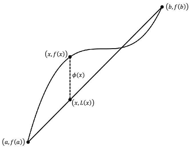
With Rolle’s Theorem in hand we can prove the MVT which is really a corollary to Rolle’s Theorem or, more precisely, it is a generalization of Rolle’s Theorem. To prove it we only need to find the right function to apply Rolle’s Theorem to. The following figure shows a function, \(f(x)\text{,}\) cut by a secant line, \(L(x)\text{,}\) from \((a, f(a))\) to \((b,f(b))\text{.}\)
The Mean Value Theorem is extraordinarily useful. Almost all of the properties of the derivative that you used in calculus follow more or less easily from it. For example the following is true.
Suppose \(c\) and \(d\) are as described in the corollary. Then by the Mean Value Theorem there is some number, say \(\alpha\in(c,d)\subseteq(a,b)\) such that
Suppose \(f\) is differentiable on some interval \((a,b)\text{,}\)\(f^\prime\) is continuous on \((a,b)\text{,}\) and that \(f^\prime(c)>0\) for some \(c\in (a,b)\text{.}\) Then there is an interval, \(I\subset (a,b)\text{,}\) containing \(c\) such that for every \(x, y\) in \(I\) where \(x\ge y\text{,}\)\(f(x)\ge f(y)\text{.}\)
Suppose that \(f\) is differentiable, and \(f^\prime \) is continuous on some interval \((a,b)\text{.}\) If \(f^\prime(c)\lt 0\) for some \(c\in
(a,b)\) then there is an interval, \(I\subset (a,b)\text{,}\) containing \(c\) such that for every \(x, y\) in \(I\) where \(x\ge y\text{,}\)\(f(x)\le f(y)\text{.}\)